

Exponential and Logarithmic Functions
COMPOSITE FUNCTIONS
For functions  and
and
 , when we enter
 on a TI-83 or TI-83 Plus we are entering the
composition
on a TI-83 or TI-83 Plus we are entering the
composition  . The composite
functions found in Section 11.1, Example 2 are checked using tables on a
graphing calculator. To check that  when
when
 and g(x) = x − 1, enter
 , and
, and  on
the equation-editor screen. We use the
on
the equation-editor screen. We use the
VARS Y-VARS menu to enter  . To do this,
position the cursor beside
. To do this,
position the cursor beside
![]() = and press
= and press .
.
Then compare the values of  and
in a table. We show a table with TblStart =
1, ΔTbl = 0.5, and Indpnt and Depend both
and
in a table. We show a table with TblStart =
1, ΔTbl = 0.5, and Indpnt and Depend both
set on Auto. Use the  key to scroll across
the table to see the
key to scroll across
the table to see the  - and
- and
 -columns.
Similarly, to check that
 , also enter
 and
and  . To
enter
. To
enter  , position the cursor beside
=
, position the cursor beside
=
and press  .
.
GRAPHING FUNCTIONS AND THEIR INVERSES
We can graph the inverse of a function using the DrawInv feature from the DRAW
menu.
Section 11.1, Example 9(c) Graph the inverse of the function g(x) = x3 +
2.
We will graph g(x), g-1(x), and the line y = x on the same screen. Press
 to go to the equation-editor screen and
clear
to go to the equation-editor screen and
clear
or deselect any existing entries. Then enter
![]() = x3 + 2 and
= x3 + 2 and
![]() = x. Select a
square window by pressing
= x. Select a
square window by pressing  5. Now paste
the DrawInv command from the DRAW DRAW menu to the home screen by pressing
 8. Indicate that we want
to draw the inverse of ![]() by pressing
by pressing
![]() 11 . Finally press
ENTER to see the graph of
11 . Finally press
ENTER to see the graph of  along with
the graphs of
along with
the graphs of ![]()
and ![]() . We show a window
that has been squared from the standard window.
. We show a window
that has been squared from the standard window.
The drawing of
can be cleared from the graph screen by pressing
![]() 1to select the
ClrDraw (clear drawing)
1to select the
ClrDraw (clear drawing)
operation. If ClrDraw was not accessed from the graph screen, it must be
followed by  . The graph will also be cleared
when another function is subsequently entered on the “Y =” screen and graphed.
GRAPHING LOGARITHMIC FUNCTIONS
Section 11.3, Example 4 Graph:  .
.
We enter y = log(x/5)+1on the equation-editor screen by positioning the cursor
beside one of the function names and pressing
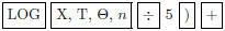 1. Note that the parentheses must be closed
in the denominator of the logarithmic function.
1. Note that the parentheses must be closed
in the denominator of the logarithmic function.
(Clear or deselect any previously entered functions.) We show the function
graphed in the window [−2, 10,−5, 5].
MORE ON GRAPHING
11.5, Example 4 Graph:  .
.
We enter  on the equation-editor screen by positioning the cursor
beside one of the function names and pressing
on the equation-editor screen by positioning the cursor
beside one of the function names and pressing
 1. (Clear or deselect any previously entered
functions.) Select a window and press
1. (Clear or deselect any previously entered
functions.) Select a window and press
 . We show the function graphed in the window
[−5, 5,−2, 10].
. We show the function graphed in the window
[−5, 5,−2, 10].
Section 11.5, Example 5(b) Graph: f(x) = ln(x + 3).
We enter y = ln(x + 3) on the equation-editor screen by positioning the cursor
beside one of the function names and pressing
 . (Clear or deselect any previously entered
functions.) Select a window and press
. (Clear or deselect any previously entered
functions.) Select a window and press
![]() . We show
. We show
the function graphed in the window [−5, 10,−5, 5].
Section 11.5, Example 6 Graph:
 .
.
To use a graphing calculator we must first change the logarithmic base to e or
10. We will use e here. Recall that the change of
base formula is 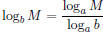 , where a and b are any
logarithmic bases and M is any positive number. Let a = e, b = 7, and
, where a and b are any
logarithmic bases and M is any positive number. Let a = e, b = 7, and
M = x and substitute in the change-of-base formula. After clearing or
deselecting previously entered functions, enter
on the equation-editor screen by positioning the cursor beside
 = and pressing
 2. Note
that the parentheses must be closed in both the numerator and the denominator.
Select a viewing window and press
![]() . We show the graph
in the window [−2, 8,−2, 5].
. We show the graph
in the window [−2, 8,−2, 5].
EXPONENTIAL REGRESSION
The STAT CALC menu contains an exponential regression feature.
Section 11.7, Example 9(a) In 1800, over 500,000 Tule elk inhabited the
state of California. By the late 1800s, after the
California Gold Rush, there were fewer than 50 elk remaining in the state. In
1978, wildlife biologists introduced a herd of 10
Tule elk into the Point Reyes National Seashore near San Francisco. By 1982, the
herd had grown to 24 elk. There were 70 elk
in 1986, 200 in 1996, and 500 in 2002. Use regression to fit an exponential
function to the data and graph the function.
We enter the data as described on page 22 of this manual. Let x represent the
number of years since 1978.
Now select ExpReg from the STAT CALC menu by pressing
 and also press
![]() 11to copy the
11to copy the
regression equation to the “Y =” screen. The calculator returns the values of a
and b for the exponential function y = abx. We
have y = 1 3.01608148(1.168547698)x. We graph the equation in the window [−2,
40,−5, 1000], Xscl = 5, Yscl = 100.
This function can be evaluated using one of the methods on page 18.