Root Finding and Nonlinear Sets of Equations

9.4 Newton-Raphson Method Using Derivative
 

Perhaps themost celebrated of all one-dimensional root-finding routines is Newton’s
method, also called the Newton-Raphson method. This method is distinguished
from the methods of previous sections by the fact that it requires the evaluation
of both the function f(x), and the derivative f'(x), at arbitrary points x. The
Newton-Raphson formula consists geometrically of extending the tangent line at a
current point until it crosses zero, then setting the next guess to the abscissa
of that zero-crossing (see Figure 9.4.1). Algebraically, the method derives from the
familiar Taylor series expansion of a function in the neighborhood of a point,

For small enough values of , and for well-behaved functions, the terms beyond
linear are unimportant, hence implies

Newton-Raphson is not restricted to one dimension. The method readily
generalizes to multiple dimensions, as we shall see in §9.6 and §9.7, below.

Far from a root, where the higher-order terms in the series are important, the
Newton-Raphson formula can give grossly inaccurate, meaningless corrections. For
instance, the initial guess for the root might be so far from the true root as to let
the search interval include a local maximum or minimum of the function. This can
be death to the method (see Figure 9.4.2). If an iteration places a trial guess near
such a local extremum, so that the first derivative nearly vanishes, then Newton-
Raphson sends its solution off to limbo, with vanishingly small hope of recovery.

Figure 9.4.1. Newton’s method extrapolates the local derivative to find the next estimate of the root. In
this example it works well and converges quadratically.

Figure 9.4.2. Unfortunate case where Newton’s method encounters a local extremum and shoots off to
outer space. Here bracketing bounds, as in rtsafe, would save the day.

Figure 9.4.3. Unfortunate case where Newton’s method enters a nonconvergent cycle. This behavior
is often encountered when the function f is obtained, in whole or in part, by table interpolation. With
a better initial guess, the method would have succeeded.

Like most powerful tools, Newton-Raphson can be destructive used in inappropriate
circumstances. Figure 9.4.3 demonstrates another possible pathology.

Why do we call Newton-Raphson powerful? The answer lies in its rate of
convergence: Within a small distance ε of x the function and its derivative are
approximately:

By the Newton-Raphson formula,

so that

When a trial solution xi differs from the true root by , we can use (9.4.3) to express
in (9.4.4) in terms of and derivatives at the root itself. The result is
a recurrence relation for the deviations of the trial solutions

Equation (9.4.6) says that Newton-Raphson converges quadratically (cf. equation
9.2.3). Near a root, the number of significant digits approximately doubles
with each step. This very strong convergence property makes Newton-Raphson the
method of choice for any function whose derivative can be evaluated efficiently, and
whose derivative is continuous and nonzero in the neighborhood of a root.

Even where Newton-Raphson is rejected for the early stages of convergence
(because of its poor global convergence properties), it is very common to “polish
up” a root with one or two steps of Newton-Raphson, which can multiply by two
or four its number of significant figures!

For an efficient realization of Newton-Raphson the user provides a routine that
evaluates both f(x) and its first derivative f'(x) at the point x. The Newton-Raphson
formula can also be applied using a numerical difference to approximate the true
local derivative,

This is not, however, a recommended procedure for the following reasons: (i) You
are doing two function evaluations per step, so at best the superlinear order of
convergence will be only . (ii) If you take dx too small you will be wiped
out by roundoff, while if you take it too large your order of convergence will be
only linear, no better than using the initial evaluation for all subsequent
steps. Therefore, Newton-Raphson with numerical derivatives is (in one dimension)
always dominated by the secant method of §9.2. (In multidimensions, where there
is a paucity of available methods, Newton-Raphson with numerical derivatives must
be taken more seriously. See §9.6–9.7.)

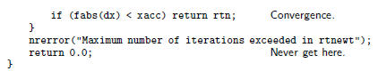
The following function calls a user supplied function funcd(x,fn,df) which
supplies the function value as fn and the derivative as df. We have included
input bounds on the root simply to be consistent with previous root-finding routines:
Newton does not adjust bounds, and works only on local information at the point
x. The bounds are used only to pick the midpoint as the first guess, and to reject
the solution if it wanders outside of the bounds.

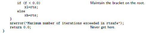
While Newton-Raphson’s global convergence properties are poor, it is fairly
easy to design a fail-safe routine that utilizes a combination of bisection and Newton-
Raphson. The hybrid algorithm takes a bisection step whenever Newton-Raphson
would take the solution out of bounds, or whenever Newton-Raphson is not reducing
the size of the brackets rapidly enough.

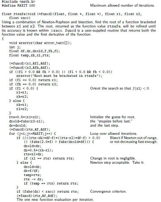
For many functions the derivative f'(x) often converges to machine accuracy
before the function f(x) itself does. When that is the case one need not subsequently
update f'(x). This shortcut is recommended only when you confidently understand
the generic behavior of your function, but it speeds computations when the derivative
calculation is laborious. (Formally thismakes the convergence only linear, but if the
derivative isn’t changing anyway, you can do no better.)

Newton-Raphson and Fractals

An interesting sidelight to our repeated warnings about Newton-Raphson’s
unpredictable global convergence properties — its very rapid local convergence
notwithstanding— is to investigate, for some particular equation, the set of starting
values from which the method does, or doesn’t converge to a root.

Consider the simple equation

whose single real root is z = 1, but which also has complex roots at the other two
cube roots of unity, exp( ±2π i=3). Newton’s method gives the iteration

Up to now, we have applied an iteration like equation (9.4.9) only for real
starting values , but in fact all of the equations in this section also apply in the
complex plane. We can therefore map out the complex plane into regions from which
a starting value , iterated in equation (9.4.9), will, or won’t, converge to z = 1.
Naively, we might expect to find a “basin of convergence” somehow surrounding
the root z = 1. We surely do not expect the basin of convergence to fill the whole
plane, because the plane must also contain regions that converge to each of the two
complex roots. In fact, by symmetry, the three regions must have identical shapes.
Perhaps they will be three symmetric 120° wedges, with one root centered in each?

Now take a look at Figure 9.4.4, which shows the result of a numerical
exploration. The basin of convergence does indeed cover 1/3 the area of the
complex plane, but its boundary is highly irregular— in fact, fractal. (A fractal, so
called, has self-similar structure that repeats on all scales of magnification.) How
does this fractal emerge from something as simple as Newton’s method, and an
equation as simple as (9.4.8)? The answer is already implicit in Figure 9.4.2, which
showed how, on the real line, a local extremum causes Newton’s method to shoot
off to infinity. Suppose one is slightly removed from such a point. Then one might
be shot off not to infinity, but — by luck — right into the basin of convergence

Figure 9.4.4. The complex z plane with real and imaginary components in the range (−2; 2). The
black region is the set of points from which Newton’s method converges to the root z = 1of the equation
z³ − 1 = 0. Its shape is fractal.

of the desired root. But that means that in the neighborhood of an extremum there
must be a tiny, perhaps distorted, copy of the basin of convergence — a kind of
“one-bounce away” copy. Similar logic shows that there can be “two-bounce”
copies, “three-bounce” copies, and so on. A fractal thus emerges.

Notice that, for equation (9.4.8), almost the whole real axis is in the domain of
convergence for the root z = 1. We say “almost” because of the peculiar discrete
points on the negative real axis whose convergence is indeterminate (see figure).
What happens if you start Newton’s method from one of these points? (Try it.)

9.5 Roots of Polynomials
 

Here we present a few methods for finding roots of polynomials. These will
serve for most practical problems involving polynomials of low-to-moderate degree
or for well-conditioned polynomials of higher degree. Not as well appreciated as it
ought to be is the fact that some polynomials are exceedingly ill-conditioned. The
tiniest changes in a polynomial’s coefficients can, in the worst case, send its roots
sprawling all over the complex plane. (An infamous example due to Wilkinson is
detailed by Acton .)

Recall that a polynomial of degree n will have n roots. The roots can be real
or complex, and they might not be distinct. If the coefficients of the polynomial are
real, then complex roots will occur in pairs that are conjugate, i.e., if = a + bi
is a root then = a − bi will also be a root. When the coefficients are complex,
the complex roots need not be related.

Multiple roots, or closely spaced roots, produce themost difficulty for numerical
algorithms (see Figure 9.5.1). For example, P(x) = (x−a)² has a double real root
at x = a. However, we cannot bracket the root by the usual technique of identifying
neighborhoods where the function changes sign, nor will slope-following methods
such as Newton-Raphson work well, because both the function and its derivative
vanish at a multiple root. Newton-Raphson may work, but slowly, since large
roundoff errors can occur. When a root is known in advance to be multiple, then
special methods of attack are readily devised. Problems arise when (as is generally
the case) we do not know in advance what pathology a root will display.

Deflation of Polynomials

When seeking several or all roots of a polynomial, the total effort can be
significantly reduced by the use of deflation. As each root r is found, the polynomial
is factored into a product involving the root and a reduced polynomial of degree
one less than the original, i.e., P(x) = (x −r)Q(x). Since the roots of Q are
exactly the remaining roots of P, the effort of finding additional roots decreases,
because we work with polynomials of lower and lower degree as we find successive
roots. Even more important, with deflation we can avoid the blunder of having our
iterative method converge twice to the same (nonmultiple) root instead of separately
to two different roots.

Deflation, which amounts to synthetic division, is a simple operation that acts
on the array of polynomial coefficients. The concise code for synthetic division by a
monomial factor was given in §5.3 above. You can deflate complex roots either by
converting that code to complex data type, or else—in the case of a polynomialwith
real coefficients but possibly complex roots— by deflating by a quadratic factor,

[x − (a + ib)] [x − (a − ib)] = x² − 2ax + (a² +b²) (9.5.1)

The routine poldiv in §5.3 can be used to divide the polynomial by this factor.