The Exponential Function

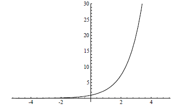
Figure 6.1.1 Graph of y = ex
Example The integral  may also be
handled by integration by parts, although
with a little more work than in the previous example. Here we will let

Then

We now perform another integration by parts by choosing

Then

At first glance it may seem that we are back to where we
started; however, all we need to
do now is solve for  . That is, we have

so

Note that we have added an arbitrary constant c since we are seeking the general antiderivative.

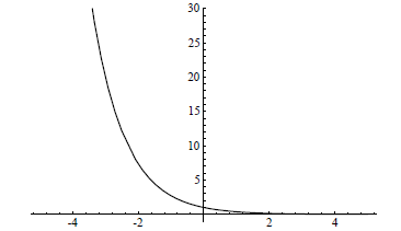
Figure 6.1.2 Graph of y = e-x
We now have sufficient information about the exponential function to understand
the
geometry of its graph. Since e > 0 , we know that ex > 0 for all
rational values of x, and
hence, by continuity, for all values of x. Since e > 1, it follows that

and

Moreover, since

and

for all x, the graph of y = ex is always
increasing and always concave up. Moreover,
(6.1.30) and (6.1.31) indicate that as x increases, the graph is not only
increasing, but its
slope is increasing at the same rate that y is increasing. Thus we should expect
y to grow
at a very rapid rate, as we see in Figure 6.1.1. This rate of growth is
characterized as
exponential growth. Figure 6.1.2 shows the graph of y = e-x , which
is the graph of y = ex
reflected about the y-axis. In this case y decreases asymptotically toward 0 as
x increases;
this is known as exponential decay
We will close this section with an application to the problem of uninhibited
population
growth, a problem we first considered in Section 1.4.
Uninhibited population growth
Recall from Section 1.4 that if  represents the size of a population after n units of time
and the population grows at a constant rate of α100% per unit of time, then
the sequence
 must satisfy the linear difference equation

for n = 0, 1, 2, . . .. At that time we saw that the solution of this equation is given by

The crucial aspect of (6.1.32) is the statement that
amount of change in the size of the
population over any unit of time is proportional to the current size of the
population.
Hence if x(t) represents the size of a population at time t, where the
population can
change continuously over time, then the continuous time analog of (6.1.32) is
the differential
equation

for all time t. If  is
the size of the population at time t = 0, then we know from our
work in this section that the only solution to this equation is the function

Hence if the size of a population is growing at a rate
which is proportional to itself, an
assumption which, as we noted in Section 1.4, is often reasonable over short
periods of
time, then the population will grow exponentially. As in Section 1.4, we refer
to such
growth as uninhibited population growth.
Example In 1970 the population of the United States was 203.3 million and
in 1980
the population was 226.5 million. Assuming an uninhibited growth model and
letting x(t)
represent the population t years after 1970, by (6.1.35) we should have

for some constant α. Since x(10) = 226.5, we can find α by solving

That is, we need to find a value for α such that

Unfortunately, solving this equation exactly requires
being able to reverse the process of
applying the exponential function. In other words, we need an inverse for the
exponential
function. We shall take up that problem in the next section; for now we may use
a
numerical approximation. You should verify that α = 0.0108 satisfies the
equation. Thus
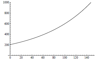
this model would predict the population of the United States t years after 1970
to be

For example, this model would predict a 1990 population of


Figure 6.1.3 Uninhibited growth model for the United
States (1970-2120)
and a population in the year 2000 of

While the prediction for 1990 is fairly accurate (the
actual population was approximately
249.6 million), the second prediction differs significantly from the Census
Bureau’s own
prediction of a population of 268.3 million for the year 2000. As we discussed
in Sections
1.4 and 1.5, an uninhibited growth model is a simple model which cannot be
expected to
be accurate for predictions too far into the future.
We shall have more to say about population models in Section 6.3, where we will
also
see another example of a differential equation. We will have a much fuller
discussion of
differential equations in Chapter 8.
Problems
1. Find the derivative of each of the following functions.

2. Evaluate each of the following integrals.


3. Find the maximum value of
 on the interval (0,∞).
4. (a) Use the Taylor series for e-x to show that
 . Hence conclude that e < 3.
(b) Show that if ![]() is
the nth order Taylor polynomial for ex at 0, then
is
the nth order Taylor polynomial for ex at 0, then

for any value of x.
(c) Use (b) to find an approximation for e with an error of less than 0.000005.
5. Find the following limits.

6. (a) Show that  for
any positive integer n.
(b) Use (a) to show that if p is any polynomial, then
 . This shows
that ex grows faster as x → ∞ than any polynomial function.
7. Graph the following functions on the specified intervals.

8. Evaluate the following improper integrals

9. Use the integral test to show that the infinite series
 converges.
10. (a) Find the Taylor series for
 .
.
(b) Use (a) to find the the Taylor series for

known as the error function.
(c) Use your result in (b) to approximate erf(1) with an error less than 0.0001.
11. Suppose x(t) is the population of a certain country t years after 1985, x(0)
= 23.4
million, and

(a) What will the population of the country be in the year 2000?
(b) In what year will the population be twice what it was in 1985?
12. Let

(a) Graph f on the interval [−5, 5].
(b) Show that f'(0) = 0.
(c) Show that  for n = 0, 1, 2, . . ..
(d) Show that f is  on (−∞,∞).
(e) Note that the Taylor series for f about 0 converges for all x in (−∞,∞), but
does
not converge to f(x) except at 0. Thus f is  on (−∞,∞), but not analytic at
0.


